5.5.5. im2col::w and im2col::w::128 modes
These modes are similar to the im2col mode with the restriction that elements are accessed across the W dimension only while keeping the H and D dimension constant.
All the constraints and rules of the im2col mode apply to these modes as well. Note that the valid Swizzling Modes must be set. In other words, swizzling mode must not be (i) no swizzle and (ii) 128-byte swizzle mode with 32-byte atomicity with 8-byte flip.
The number of elements accessed in the im2col::w::128 mode is fixed and is equal to 128. The number of elements accessed in the im2col::w mode depends on the Pixels-per-Column field in the TensorMap.
5.5.5.1. Bounding Box
In these modes, the size of the bounding box in D and H dimensions are 1.
The D and H dimensions in the tensor coordinates argument in the PTX instruction specify the position of the bounding box in the tensor space.
The Bounding-Box Lower-Corner-W and Bounding-Box Upper-Corner-W specify the two opposite corners of the Bounding Box in the W dimension.
The W dimension in the tensor coordinates argument in the PTX instruction specify the location of the first element that is to be accessed in the bounding box.
Number of pixels loaded in im2col::w mode is as specified by Pixels-per-Column in the TensorMap. Number of pixels loaded in im2col::w::128 mode is always 128. So, Pixels-per-Column is ignored in im2col::w::128 mode.
Figure 16 shows an example of the im2col::w and im2col::w::128 modes.
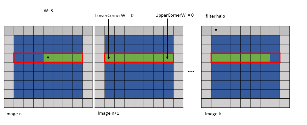
Figure 16 im2col::w and im2col::w::128 modes example
The first element can lie outside of the Bounding Box in the W-dimension only and only on the left side of the Bounding Box. Figure 17 shows an example of this.
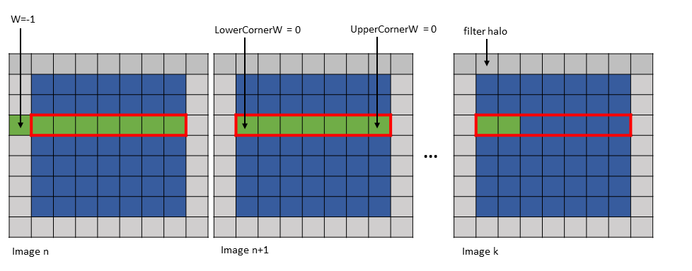
Figure 17 im2col::w and im2col::w::128 modes first element outside Bounding Box example
5.5.5.2. Traversal Stride
This is similar to im2col mode with the exception that the number of elements traversed along only the W dimension is strided by the traversal stride as specified in the TensorMap.
5.5.5.3. wHalo
In im2col::w mode, the wHalo argument in the PTX instruction specifies how many filter halo elements must be loaded at the end of the image.
In im2col::w::128 mode, the halo elements are loaded after every 32 elements in the bounding box along the W dimension. The wHalo argument in the PTX instruction specifies how many halo elements must be loaded after every 32 elements.
Following is an example of .im2col::w mode access:
Tensor Size [0] = 128
Tensor Size [1] = 9
Tensor Size [2] = 7
Tensor Size [3] = 64
Pixels-per-column = 128
Channels-per-pixel = 64
Bounding Box Lower Corner W = 0
Bounding Box Upper Corner W = 0

Tensor Coordinates in the instruction = (7, 2, 3, 0)
wHalo in the instruction = 2 (as 3x3 convolution filter is used)
A tensor copy operation with the above parameters loads 128 pixels and the two halo pixels as shown in Figure 18.
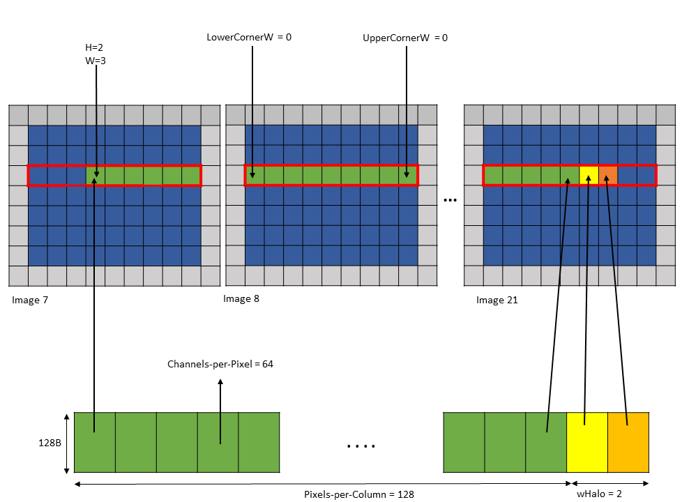
Figure 18 tensor copy operation with im2col::w mode example
The halo pixels are always loaded in the shared memory next to the main row pixels as shown in Figure 18.
Following is an example of .im2col::w::128 mode access:
Tensor Size [0] = 128
Tensor Size [1] = 9
Tensor Size [2] = 7
Tensor Size [3] = 64
Channels-per-pixel = 64
Bounding Box Lower Corner W = 0
Bounding Box Upper Corner W = 0

Tensor Coordinates in the instruction = (7, 2, 3, 0)
wHalo in the instruction = 2 (as 3x3 convolution filter is used)
A tensor copy operation with the above parameters loads 128 elements such that after every 32 elements, wHalo number of elements are loaded as shown in Figure 19.
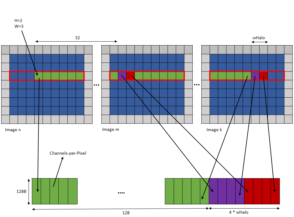
Figure 19 tensor copy operation with im2col::w::128 mode example
5.5.5.4. wOffset
In the convolution calculations, the same elements along the W dimension are reused for different locations within the convolution filter footprint. Based on the number of times a pixel is used, the pixels may be loaded into different shared memory buffers. Each buffer can be loaded by a separate tensor copy operation.
The wOffset argument in the tensor copy and prefetch instruction adjusts the source pixel location for each buffer. The exact position of the buffer is adjusted along the W dimension using the following formula:
Bounding Box Lower Corner W += wOffset
Bounding Box Upper Corner W += wOffset
W += wOffset
Following are examples of tensor copy to multiple buffers with various wHalo and wOffset values:
Example 1:
Tensor Size [0] = 128
Tensor Size [1] = 9
Tensor Size [2] = 67
Tensor Size [3] = 64
Pixels-per-Column = 128
Channels-per-pixel = 64
Bounding Box Lower Corner W = -1
Bounding Box Upper Corner W = 0
Traversal Stride = 2

Tensor Coordinates in the instruction = (7, 2, -1, 0)

Shared memory buffer 1:
   wHalo = 1
   wOffset = 0

Shared memory buffer 2:
   wHalo = 0
   wOffset = 1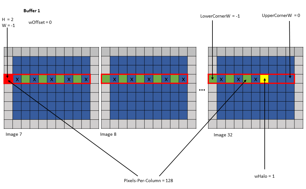
Figure 20 tensor copy operation to buffer 1 of Example 1
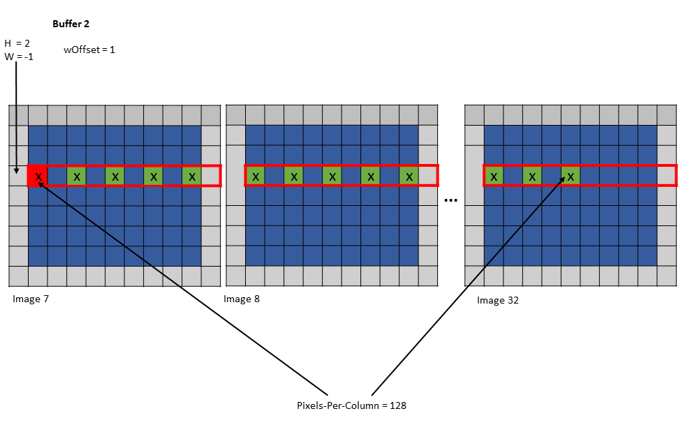
Figure 21 tensor copy operation to buffer 2 of Example 1
Example 2:
Tensor Size [0] = 128
Tensor Size [1] = 7
Tensor Size [2] = 7
Tensor Size [3] = 64
Pixels-per-Column = 128
Channels-per-pixel = 64
Bounding Box Lower Corner W = -1
Bounding Box Upper Corner W = -1
Traversal Stride = 3

Tensor Coordinates in the instruction = (7, 2, -1, 0)

Shared memory buffer 1:
   wHalo = 0
   wOffset = 0

Shared memory buffer 2:
   wHalo = 0
   wOffset = 1

Shared memory buffer 3:
   wHalo = 0
   wOffset = 2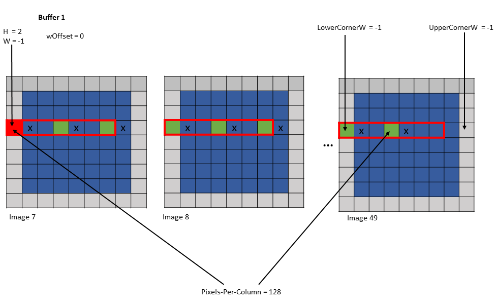
Figure 22 tensor copy operation to buffer 1 of Example 2
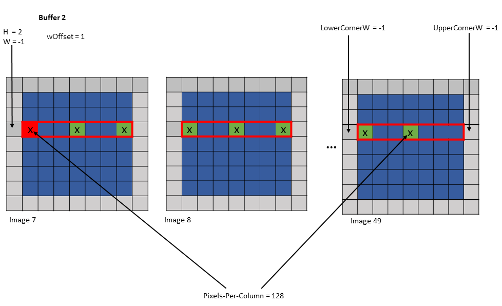
Figure 23 tensor copy operation to buffer 2 of Example 2
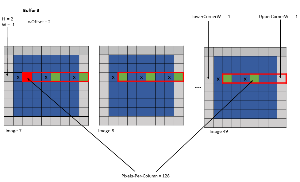
Figure 24 tensor copy operation to buffer 3 of Example 2
5.5.6. Interleave layout
Tensor can be interleaved and the following interleave layouts are supported:
- No interleave (NDHWC)
- 8 byte interleave (NC/8DHWC8): C8 utilizes 16 bytes in memory assuming 2B per channel.
- 16 byte interleave (NC/16HWC16): C16 utilizes 32 bytes in memory assuming 4B per channel.
The C information is organized in slices where sequential C elements are grouped in 16 byte or 32 byte quantities.
If the total number of channels is not a multiple of the number of channels per slice, then the last slice must be padded with zeros to make it complete 16B or 32B slice.
Interleaved layouts are supported only for the dimensionalities: 3D, 4D and 5D.
The interleave layout is not supported for .im2col::w and .im2col::w::128 modes.
5.5.7. Swizzling Modes
The layout of the data in the shared memory can be different to that of global memory, for access performance reasons. The following describes various swizzling modes:
No swizzle mode:
There is no swizzling in this mode and the destination data layout is exactly similar to the source data layout.
| 0 | 1 | 2 | 3 | 4 | 5 | 6 | 7 |
|---|---|---|---|---|---|---|---|
| 0 | 1 | 2 | 3 | 4 | 5 | 6 | 7 |
… Pattern repeats …
32 byte swizzle mode:
The following table, where each element (numbered cell) is 16 byte and the starting address is 256 bytes aligned, shows the pattern of the destination data layout:
| 0 | 1 | 2 | 3 | 4 | 5 | 6 | 7 |
|---|---|---|---|---|---|---|---|
| 1 | 0 | 3 | 2 | 5 | 4 | 7 | 6 |
… Pattern repeats …
An example of the 32 byte swizzle mode for NC/(32B)HWC(32B) tensor of 1x2x10x10xC16 dimension, with the innermost dimension holding slice of 16 channels with 2 byte/channel, is shown in Figure 25.
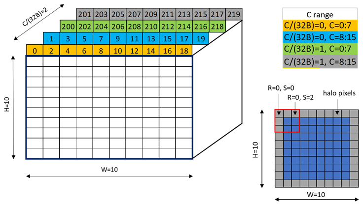
Figure 25 32-byte swizzle mode example
Figure 26 shows the two fragments of the tensor: one for C/(32B) = 0 and another for C/(32B) = 1.
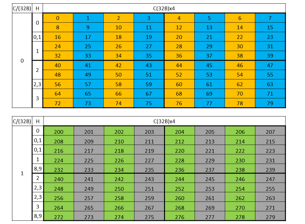
Figure 26 32-byte swizzle mode fragments
Figure 27 shows the destination data layout with 32 byte swizzling.
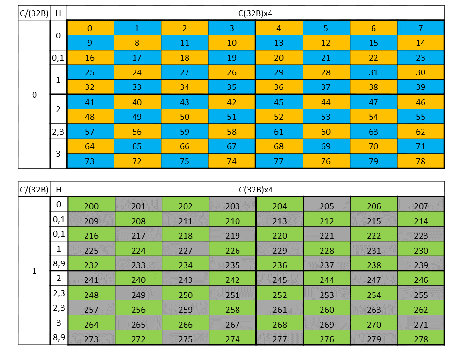
Figure 27 32-byte swizzle mode destination data layout
64 byte swizzle mode:
The following table, where each element (numbered cell) is 16 byte and the starting address is 512 bytes aligned, shows the pattern of the destination data layout:
| 0 | 1 | 2 | 3 | 4 | 5 | 6 | 7 |
|---|---|---|---|---|---|---|---|
| 1 | 0 | 3 | 2 | 5 | 4 | 7 | 6 |
| 2 | 3 | 0 | 1 | 6 | 7 | 4 | 5 |
| 3 | 2 | 1 | 0 | 7 | 6 | 5 | 4 |
… Pattern repeats …
An example of the 64 byte swizzle mode for NHWC tensor of 1x10x10x64 dimension, with 2 bytes / channel and 32 channels, is shown in Figure 28.
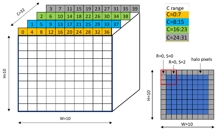
Figure 28 64-byte swizzle mode example
Each colored cell represents 8 channels. Figure 29 shows the source data layout.
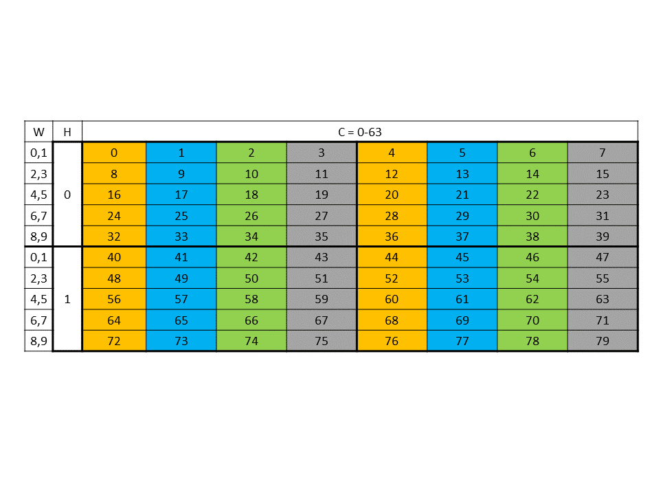
Figure 29 64-byte swizzle mode source data layout
Figure 30 shows the destination data layout with 64 byte swizzling.
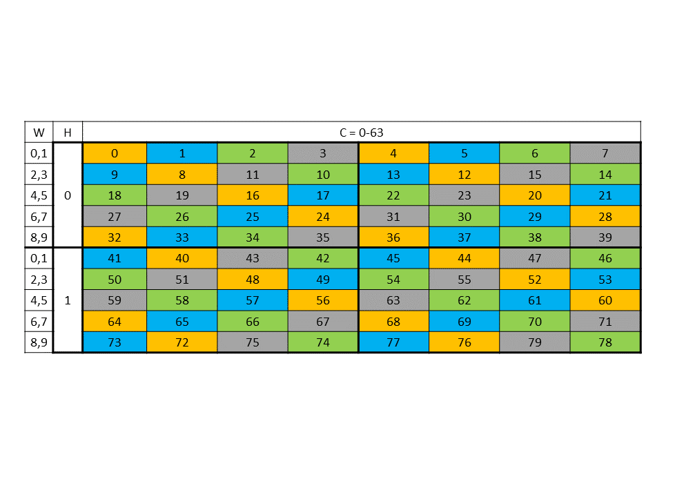
Figure 30 64-byte swizzle mode destination data layout
96 byte swizzle mode:
The following table where each element (numbered cell) is 16 byte shows the swizzling pattern at the destination data layout:
| 0 | 1 | 2 | 3 | 4 | 5 | 6 | 7 |
|---|---|---|---|---|---|---|---|
| 1 | 0 | 3 | 2 | 5 | 4 | 7 | 6 |
… Pattern repeats …
An example of the data layout in global memory and its swizzled data layout in shared memory where each element (colored cell) is 16 bytes and the starting address is 256 bytes aligned is shown in Figure 31.
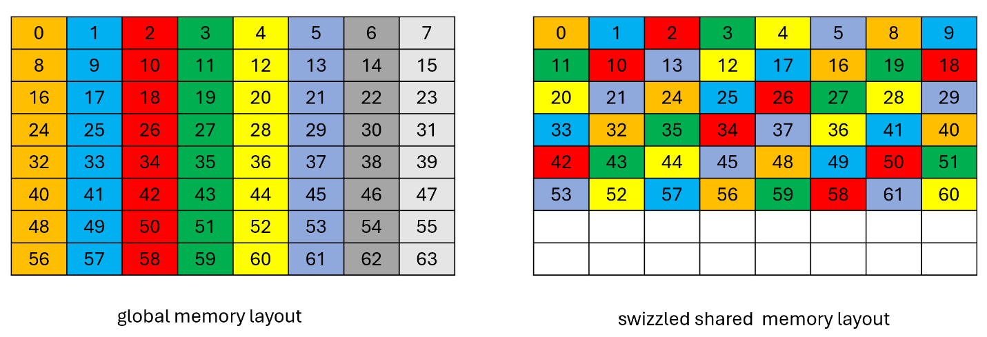
Figure 31 96-byte swizzle mode example
128 byte swizzle mode:
The 128-byte swizzling mode supports the following sub-modes:
16-byte atomicity sub-mode:
In this sub-mode, the 16-byte of data is kept intact while swizzling.
The following table, where each element (numbered cell) is 16 byte and the starting address is 1024 bytes aligned, shows the pattern of the destination data layout:
| 0 | 1 | 2 | 3 | 4 | 5 | 6 | 7 |
|---|---|---|---|---|---|---|---|
| 1 | 0 | 3 | 2 | 5 | 4 | 7 | 6 |
| 2 | 3 | 0 | 1 | 6 | 7 | 4 | 5 |
| 3 | 2 | 1 | 0 | 7 | 6 | 5 | 4 |
| 4 | 5 | 6 | 7 | 0 | 1 | 2 | 3 |
| 5 | 4 | 7 | 6 | 1 | 0 | 3 | 2 |
| 6 | 7 | 4 | 5 | 2 | 3 | 0 | 1 |
| 7 | 6 | 5 | 4 | 3 | 2 | 1 | 0 |
… Pattern repeats …
An example of the 128 byte swizzle mode for NHWC tensor of 1x10x10x64 dimension, with 2 bytes / channel and 64 channels, is shown in Figure 32.
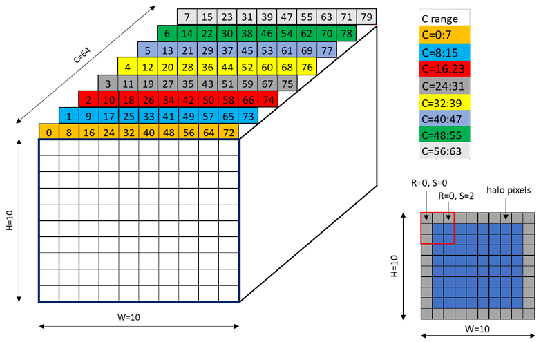
Figure 32 128-byte swizzle mode example
Each colored cell represents 8 channels. Figure 33 shows the source data layout.
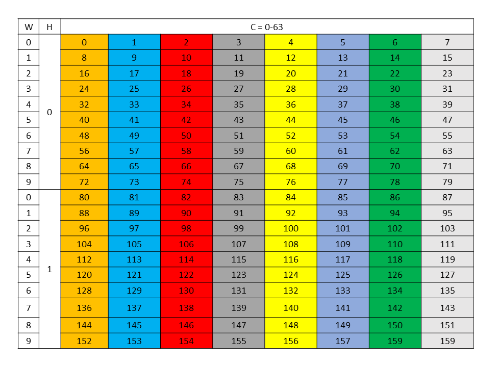
Figure 33 128-byte swizzle mode source data layout
Figure 34 shows the destination data layout with 128 byte swizzling.
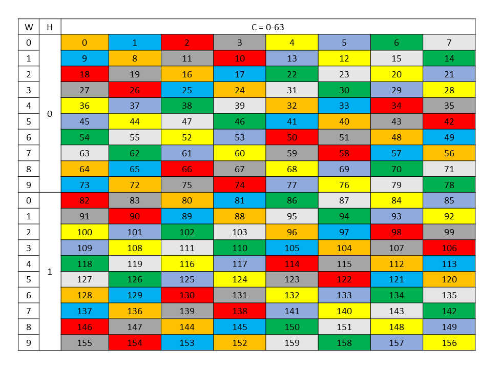
Figure 34 128-byte swizzle mode destination data layout
32-byte atomicity sub-mode:
In this sub-mode, the 32-byte of data is kept intact while swizzling.
The following table where each element (numbered cell) is 16 byte shows the swizzling pattern at the destination data layout:
| 0 1 | 2 3 | 4 5 | 6 7 |
|---|---|---|---|
| 2 3 | 0 1 | 6 7 | 4 5 |
| 4 5 | 6 7 | 0 1 | 2 3 |
| 6 7 | 4 5 | 2 3 | 0 1 |
… Pattern repeats …
This sub-mode requires 32 byte alignment at shared memory.
An example of the data layout in global memory and its swizzled data layout in shared memory where each element (colored cell) is 16 bytes is shown in Figure 35.
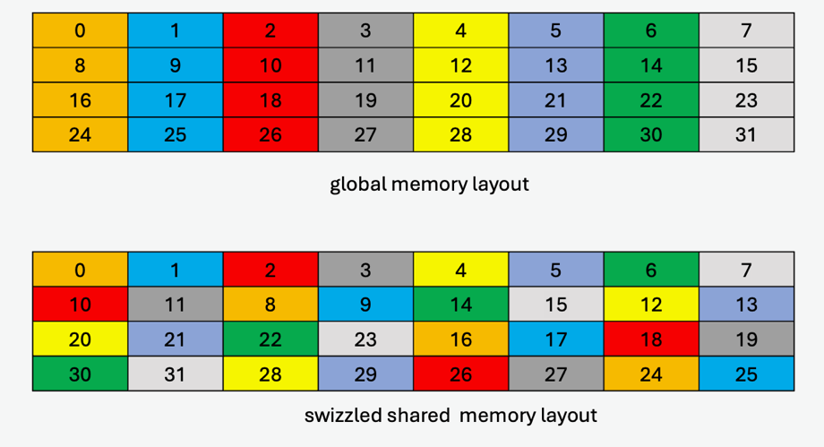
Figure 35 128-byte swizzle mode example with 32-byte atomicity
32-byte atomicity with 8-byte flip sub-mode:
The swizzling pattern for this sub-mode is similar to the 32-byte atomicity sub-mode except that there is a flip of adjacent 8-bytes within the 16-byte data at every alternate shared memory line. Note that this mode is legal only when cp.async.bulk.tensor specifies the copy direction as .shared::cluster.global or otherwise .shared::cta.global.
An example of the data layout in global memory and its swizzled data layout in shared memory where each element (colored cell) is 16 bytes (two 8-byte sub-elements for each 16-byte colored cell are shown to show the flip) is shown in Figure 36.
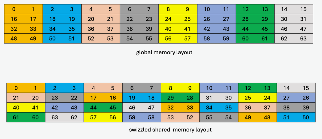
Figure 36 128-byte swizzle mode example with 32-byte atomicity with 8-byte flip
64-byte atomicity sub-mode:
In this sub-mode, the 64-byte of data is kept intact while swizzling.
The following table where each element (numbered cell) is 16 byte shows the swizzling pattern at the destination data layout:
| 0 1 2 3 | 4 5 6 7 |
|---|---|
| 4 5 6 7 | 0 1 2 3 |
… Pattern repeats …
This sub-mode requires 64-byte alignment at shared memory.
An example of the data layout in global memory and its swizzled data layout in shared memory where each element (colored cell) is 16 bytes is shown in Figure 37.
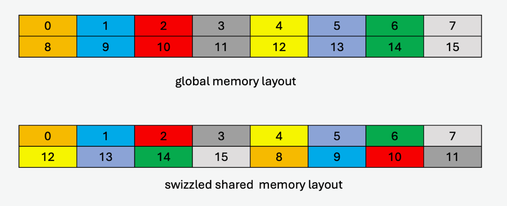
Figure 37 128-byte swizzle mode example with 64-byte atomicity
Table 14 lists the valid combination of swizzle-atomicity with the swizzling-mode.
Table 14 Valid combination of swizzle-atomicity with swizzling-mode
| Swizzling Mode | Swizzle-Atomicity |
|---|---|
| No Swizzling | – |
| 32B Swizzling Mode | 16B |
| 64B Swizzling Mode | 16B |
| 96B Swizzling Mode | 16B |
| 128B Swizzling Mode | 16B, 32B, 32B + 8B-flip, 64B |
The value of swizzle base offset is 0 when the dstMem shared memory address is located at the following boundary:
| Swizzling Mode | Starting address of the repeating pattern |
|---|---|
| 128-Byte swizzle | 1024-Byte boundary |
| 96-Byte swizzle | 256-Byte boundary |
| 64-Byte swizzle | 512-Byte boundary |
| 32-Byte swizzle | 256-Byte boundary |
Otherwise, the swizzle base offset is a non-zero value, computed using the following formula:
| Swizzling Mode | Formula |
|---|---|
| 128-Byte swizzle | base offset = (dstMem / 128) % 8 |
| 96-Byte swizzle | base offset = (dstMem / 128) % 2 |
| 64-Byte swizzle | base offset = (dstMem / 128) % 4 |
| 32-Byte swizzle | base offset = (dstMem / 128) % 2 |
5.5.8. Tensor-map
The tensor-map is a 128-byte opaque object either in .const space or .param (kernel function parameter) space or .global space which describes the tensor properties and the access properties of the tensor data described in previous sections.
Tensor-Map can be created using CUDA APIs. Refer to CUDA programming guide for more details.